Agenda
Part A -- The mixing scenario: a mass balance becomes an ODE (Sec. 2.1)
Part B -- The heating vessel: the energy balance (Sec. 2.1)
Part C -- Laplace transforms and the three-step method (Sec. 2.2-2.3)
Part D -- Inversion by partial fractions; what the roots tell us (Ch. 3)
Setup (run once)
- SymPy for the algebra, NumPy/SciPy for numbers, Matplotlib to plot
import numpy as np
import matplotlib.pyplot as plt
import sympy as sp
from scipy.integrate import solve_ivp
plt.rcParams.update({"font.size": 15})
t, s = sp.symbols("t s", positive=True)
Introduce -- the 3:00 PM shift change (Sec. 2.1)
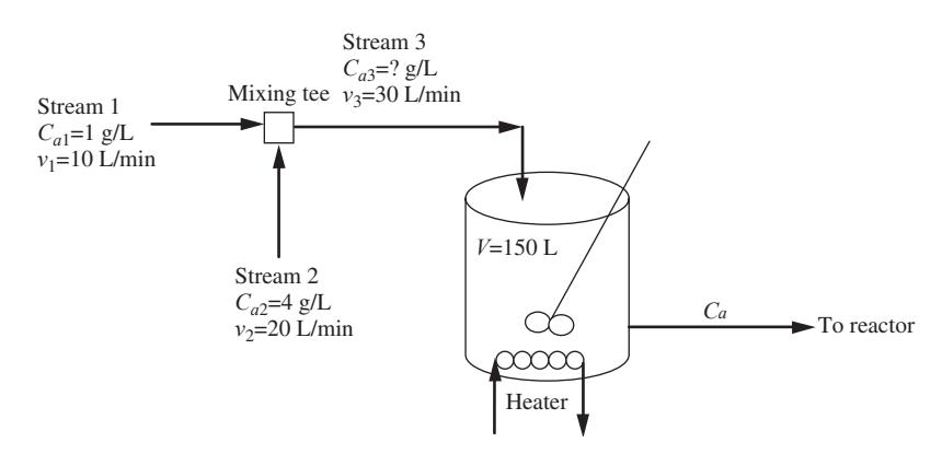
- Stream 1: 10 L/min at 1 g/L. Stream 2: 20 L/min at 4 g/L.
- They meet in a tee and feed a heating vessel ($\tau = 5$ min).
- At 3:00 PM a new operator swaps the two flow rates.
- At 3:30 PM the reactor misbehaves. What happened to the vessel's exit concentration over that half hour?
Derive 1/3 -- component balance on the tee
No holdup in a tee: rate in = rate out.
$$v_1C_{a1} + v_2C_{a2} = v_3C_{a3}$$
Before: $(10)(1) + (20)(4) = 30\,C_{a3} \Rightarrow C_{a3} = 3$ g/L. After: $(20)(1) + (10)(4) = 30\,C_{a3} \Rightarrow C_{a3} = 2$ g/L.
Derive 2/3 -- unsteady balance on the vessel
In $-$ out $=$ accumulation, constant $V$ and $v_3$:
$$v_3C_{a3} - v_3C_a = \frac{d}{dt}(VC_a) \;\Rightarrow\; \frac{V}{v_3}\frac{dC_a}{dt} + C_a = C_{a3} \qquad (2.1)$$
$\tau = V/v_3 = 5$ min (so $V = 150$ L).
Derive 3/3 -- separate and integrate
$5\,dC_a/dt + C_a = 2$ with $C_a(0) = 3$ g/L:
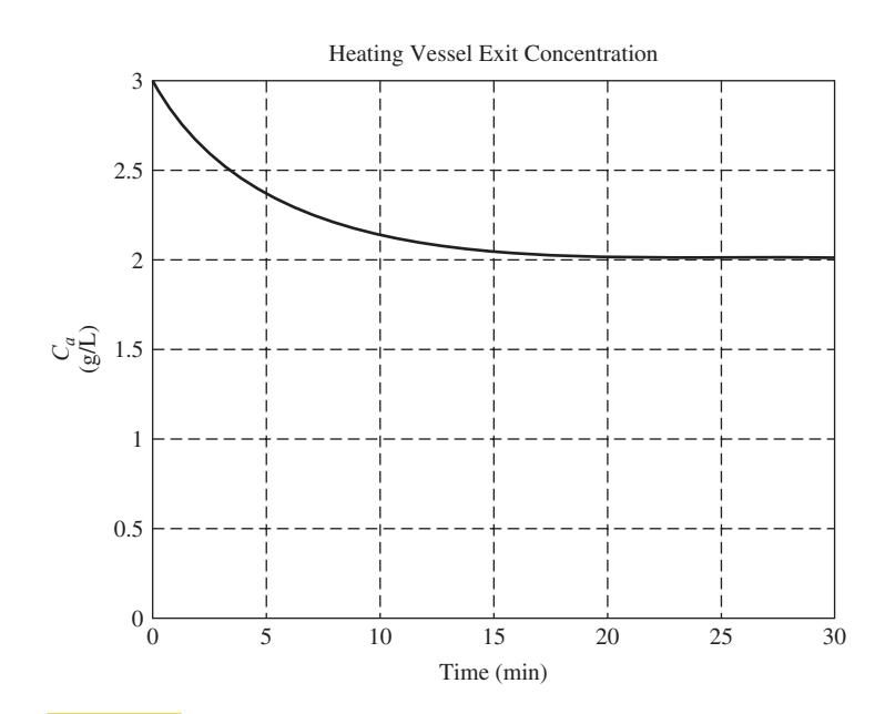
$$\int_3^{C_a}\frac{dC_a}{2 - C_a} = \int_0^t\frac{dt}{5} \;\Rightarrow\; C_a = 2 + e^{-t/5} \qquad (2.2)$$
Code 1/3 -- the tee balance as a function
- Mirrors Derive 1/3: solve the balance for the outlet
- Returns two values: outlet flow and outlet composition
def tee(v1, x1, v2, x2):
    v3 = v1 + v2                       # total flow
    return v3, (v1 * x1 + v2 * x2) / v3

print("before:", tee(10, 1, 20, 4))    # (30, 3.0)
print("after: ", tee(20, 1, 10, 4))    # (30, 2.0)
before: (30, 3.0)
after:  (30, 2.0)
Code 2/3 -- the vessel balance, symbolically
- Mirrors Derive 2/3: type the balance, let SymPy rearrange it
sp.solve(..., dC)isolates the derivative
V, v3, Ca3 = sp.symbols("V v_3 C_a3", positive=True)
Ca = sp.Function("C_a")
dC = sp.Symbol("dC")                       # stands for dC_a/dt
balance = sp.Eq(v3*Ca3 - v3*Ca(t), V*dC)   # in - out = accum.
rate = sp.solve(balance, dC)[0]
print(sp.simplify(rate))                    # v3 (C_a3 - C_a)/V
print("tau =", sp.Rational(150, 30), "min")
v_3*(C_a3 - C_a(t))/V
tau = 5 min
Code 3/3 -- solve the ODE with its initial condition
- Mirrors Derive 3/3:
dsolvereplaces separation of variables ics={...}supplies $C_a(0) = 3$ g/L
ode = sp.Eq(5 * Ca(t).diff(t) + Ca(t), 2)       # Eq. 2.1, numbers
Ca_t = sp.dsolve(ode, Ca(t), ics={Ca(0): 3}).rhs
print(Ca_t)                                     # Eq. 2.2
print(sp.simplify(5*Ca_t.diff(t) + Ca_t - 2))   # 0: it satisfies
2 + exp(-t/5)
0
Build on it -- a numerical solution that knows no calculus
solve_ivpintegrates the ODE step by step from $C_a(0)$- Compare with Eq. 2.2 at every point
def vessel(t, C, Cin):
    return [(Cin - C[0]) / 5.0]        # Eq. 2.1: dC/dt

tt = np.linspace(0, 30, 61)            # 3:00 to 3:30 PM
num = solve_ivp(vessel, [0, 30], [3.0], args=(2.0,),
                t_eval=tt, rtol=1e-8).y[0]
exact = 2 + np.exp(-tt / 5)            # Eq. 2.2
print(f"max |numerical - exact| = {np.abs(num - exact).max():.1e}")
print(f"C_a at 3:30 PM = {num[-1]:.4f} g/L")
max |numerical - exact| = 2.5e-07
C_a at 3:30 PM = 2.0025 g/L
Plot -- the operator-induced transient (cf. Fig. 2-3)
- Exact solution as a line, numerical solution as dots
fig, ax = plt.subplots(figsize=(7, 5.25))
ax.plot(tt, exact, label="Eq. 2.2, exact")
ax.plot(tt[::4], num[::4], "o", label="solve_ivp")
ax.axhline(2, ls="--", c="gray")
ax.set(xlabel="minutes after 3:00 PM", ylabel="C_a (g/L)")
ax.legend(loc="upper right")
plt.show()

Your Turn (10 min)
Prob. 2.9. Instead, at 3:00 PM the operator increases stream 1 to 20 L/min; stream 2 (20 L/min, 4 g/L) is unchanged; $V = 150$ L.
- By hand: the new $v_3$, $C_{a3}$ and $\tau$.
- Read the code: what does this print?
v3, Ca3 = tee(20, 1, 20, 4)
print(v3, Ca3, 150 / v3)
Check -- cold-call
In the book's swap, $\tau$ stayed at 5 min. In Prob. 2.9 it fell to 3.75 min. Which single quantity decides whether $\tau$ changes?
Introduce -- the same scenario, now for temperature
- Stream 1 at 25 C, stream 2 at 55 C. The heater brings the vessel outlet to 80 C.
- After the swap, with the heater unchanged: what does the reactor feed temperature do?
Derive 1/3 -- energy balance on the tee
Constant $\rho$ and $C_p$; enthalpy relative to $T_{ref}$:
$$v_1T_1 + v_2T_2 = v_3T_3 \;\Rightarrow\; T_3 = \frac{(10)(25) + (20)(55)}{30} = 45\ ^\circ\text{C}$$
After the swap: $T_3 = [(20)(25) + (10)(55)]/30 = 35$ C.
Derive 2/3 -- the heater duty at steady state
Vessel: in + heat = out:
$$Q = \rho v_3C_p(T - T_3) = (1000)(30)(1)(80 - 45) = 1.05\times10^6\ \text{cal/min} = 73.2\ \text{kW}$$
Derive 3/3 -- unsteady energy balance
Add accumulation $\frac{d}{dt}[\rho VC_p(T - T_{ref})]$ and divide by $\rho v_3 C_p$:
$$\tau\frac{dT}{dt} + T = T_3 + \frac{Q}{\rho v_3C_p} \qquad (2.3)$$
$5\,dT/dt + T = 35 + 35 = 70$, $T(0) = 80$: $\;T = 70 + 10e^{-t/5}$ (2.4).
Code 1/3 -- the tee function again, for temperatures
- Mirrors Derive 1/3: same balance, temperatures instead of $C$
- No new code: the algebra is identical
print("T3 before:", tee(10, 25, 20, 55)[1], "C")
print("T3 after: ", tee(20, 25, 10, 55)[1], "C")
T3 before: 45.0 C
T3 after:  35.0 C
Code 2/3 -- heater duty, with units
- Mirrors Derive 2/3; then convert cal/min to kW
- 1 cal = 4.184 J; 1 min = 60 s
rho, Cp, v3n = 1000.0, 1.0, 30.0      # g/L, cal/(g C), L/min
Q = rho * v3n * Cp * (80 - 45)        # cal/min
print(f"Q = {Q:.3g} cal/min = {Q * 4.184 / 60 / 1000:.1f} kW")
Q = 1.05e+06 cal/min = 73.2 kW
Code 3/3 -- solve Eq. 2.3 after the swap
- Mirrors Derive 3/3:
dsolvewith $T(0) = 80$ C
T = sp.Function("T")
heat = sp.Rational(35)                     # Q/(rho v3 Cp), C
ode_T = sp.Eq(5 * T(t).diff(t) + T(t), 35 + heat)
T_t = sp.dsolve(ode_T, T(t), ics={T(0): 80}).rhs
print(T_t)                                 # Eq. 2.4
70 + 10*exp(-t/5)
Build on it -- what heater duty restores 80 C?
- Steady state: $Q = \rho v_3 C_p (80 - T_3)$ with $T_3 = 35$ C
- Simulate: the heater is raised at $t = 10$ min
Q_new = rho * v3n * Cp * (80 - 35)           # cal/min
def heater(t, T, Q_of_t):
    return [(35 - T[0] + Q_of_t(t) / (rho*v3n*Cp)) / 5]
Q_sched = lambda t: Q if t < 10 else Q_new   # raise at 10 min
tt2 = np.linspace(0, 40, 401)
T_sim = solve_ivp(heater, [0, 40], [80.0], args=(Q_sched,),
                  t_eval=tt2, max_step=0.1).y[0]
print(f"Q_new = {Q_new:.3g} cal/min = "
      f"{Q_new * 4.184 / 60000:.1f} kW; T(40) = {T_sim[-1]:.2f} C")
Q_new = 1.35e+06 cal/min = 94.1 kW; T(40) = 79.98 C
Plot -- disturbance, then a manual correction
- The feed cools at $t = 0$; the heater is raised at $t = 10$
fig, ax = plt.subplots(figsize=(7, 5.25))
ax.plot(tt2, T_sim)
ax.plot(tt2, 70 + 10 * np.exp(-tt2 / 5), "--",
        label="no correction (Eq. 2.4)")
ax.axvline(10, ls=":", c="k")
ax.set(xlabel="minutes after 3:00 PM", ylabel="T (C)")
ax.legend(loc="lower right")
plt.show()

Your Turn (8 min)
Prob. 2.9, energy part: stream 1 rises to 20 L/min at 25 C, stream 2 stays 20 L/min at 55 C, $Q = 1.05\times10^6$ cal/min.
- By hand: the new $T_3$, $\tau$, and final outlet temperature.
- Read the code: what does this print?
print(tee(20, 25, 20, 55)[1] + 1.05e6 / (1000 * 40))
Check -- think-pair-share
The concentration and the temperature responses have exactly the same shape. Is that a coincidence of the numbers, or does it follow from Eq. 2.1 and Eq. 2.3? What would make them differ?
Introduce -- why transform at all?
- Separation of variables worked once. Higher-order models will not separate.
- The Laplace transform turns differentiation into multiplication by $s$ -- an ODE becomes algebra.
- Definition (Eq. 2.5): $F(s) = \int_0^\infty f(t)\,e^{-st}\,dt$
Derive 1/3 -- the transform of a step (Ex. 2.1)
Apply the definition to $f(t) = 1$:
$$F(s) = \int_0^\infty e^{-st}dt = -\frac{e^{-st}}{s}\Big|_0^\infty = \frac{1}{s}$$
Derive 2/3 -- the transform of a derivative
Integrate by parts, $u = e^{-st}$, $dv = f'\,dt$:
$$\mathcal{L}\left\{\frac{df}{dt}\right\} = sF(s) - f(0) \qquad (2.6)$$
The initial condition enters here, and only here.
Derive 3/3 -- transform the mixing balance
$5\,dC_a/dt + C_a = 2$, $C_a(0) = 3$:
$$5[sC_a(s) - 3] + C_a(s) = \frac{2}{s} \;\Rightarrow\; C_a(s) = \frac{2}{s(5s+1)} + \frac{15}{5s+1} \qquad (2.10)$$
Code 1/3 -- the definition, then the table
- Mirrors Derive 1/3:
sp.integratethe definition directly - Then
sp.laplace_transformreproduces Table 2.1 entries
a, k = sp.symbols("a k", positive=True)
print(sp.integrate(sp.exp(-s * t), (t, 0, sp.oo)))   # 1/s
for f in [sp.exp(-a * t), t, sp.sin(k * t), sp.cos(k * t)]:
    F = sp.laplace_transform(f, t, s, noconds=True)
    print(f, "->", F)
1/s
exp(-a*t) -> 1/(a + s)
t -> s**(-2)
sin(k*t) -> k/(k**2 + s**2)
cos(k*t) -> s/(k**2 + s**2)
Code 2/3 -- the derivative rule, checked
- Mirrors Derive 2/3 on a concrete function
- Left: transform of $f'$. Right: $sF(s) - f(0)$
f = 3 * sp.exp(-2 * t) + t                  # any test function
lhs = sp.laplace_transform(f.diff(t), t, s, noconds=True)
F = sp.laplace_transform(f, t, s, noconds=True)
rhs = s * F - f.subs(t, 0)                  # Eq. 2.6
print(sp.simplify(lhs - rhs))               # 0
0
Code 3/3 -- the three-step method, step 2
- Mirrors Derive 3/3: transform each side, solve for $C_a(s)$
- The symbol
Csstands for $C_a(s)$
Cs = sp.Symbol("C_s")
step1 = sp.Eq(5 * (s * Cs - 3) + Cs, 2 / s)   # Eq. 2.6 used
Ca_s = sp.solve(step1, Cs)[0]
print(sp.apart(Ca_s, s))
print(sp.simplify(Ca_s - (2/(s*(5*s+1)) + 15/(5*s+1))))
5/(5*s + 1) + 2/s
0
Build on it -- Example 2.2, third order
- A third-order ODE, all initial conditions zero
- By hand: three derivative transforms. Here: one line each
x = sp.Function("x")
ode3 = sp.Eq(x(t).diff(t, 3) + 4*x(t).diff(t, 2)
             + 5*x(t).diff(t) + 2*x(t), 2)
x_t = sp.dsolve(ode3, x(t), ics={x(0): 0, x(t).diff(t).subs(t, 0): 0,
                                 x(t).diff(t, 2).subs(t, 0): 0}).rhs
print(sp.expand(x_t))                          # Eq. 2.8
print(sp.apart(sp.laplace_transform(x_t, t, s, noconds=True), s))
-2*t*exp(-t) + 1 - exp(-2*t)
-1/(s + 2) - 2/(s + 1)**2 + 1/s
Your Turn (8 min)
Ex. 2.4. Solve $dx/dt + 3x = 0$, $x(0) = 2$, by the three steps.
- By hand: $x(s)$, then $x(t)$.
- Read the code: what does this print?
print(sp.laplace_transform(t**2, t, s, noconds=True))
Check -- cold-call
In the three-step method, at which step do the initial conditions enter -- and what does that imply about the form of the solution?
Introduce -- the third step: back to the time domain
- $x(s)$ rarely appears in Table 2.1 as it stands.
- Split it into simple fractions that do: partial fractions.
- Distinct real roots: Heaviside cover-up. Complex roots: keep the quadratic, complete the square. Repeated roots: match coefficients.
Derive 1/4 -- Ex. 3.1, the cover-up rule
$dx/dt + x = 1$, $x(0) = 0$ gives $x(s) = 1/[s(s+1)]$:
$$\frac{1}{s(s+1)} = \frac{A}{s} + \frac{B}{s+1}: \quad A = \frac{1}{0+1} = 1,\;\; B = \frac{1}{-1} = -1$$
$$x(t) = 1 - e^{-t} \qquad (3.6)$$
Derive 2/4 -- Ex. 3.2, the mixing scenario inverted
Eq. 2.10, with $5s + 1 = 5(s + \frac15)$:
$$C_a(s) = \frac{2}{s} - \frac{2}{s+\frac15} + \frac{3}{s+\frac15} = \frac{2}{s} + \frac{1}{s+\frac15} \;\Rightarrow\; C_a(t) = 2 + e^{-t/5}$$
The same answer as Part A, by a different road.
Derive 3/4 -- Ex. 3.4, complex roots
$x'' + 2x' + 2x = 2$, zero ICs: $x(s) = 2/[s(s^2+2s+2)]$, roots $-1 \pm j$:
$$x(s) = \frac{1}{s} - \frac{(s+1) + 1}{(s+1)^2 + 1^2} \;\Rightarrow\; x(t) = 1 - e^{-t}(\cos t + \sin t)$$
Derive 4/4 -- Ex. 3.5, a repeated root
$x(s) = 1/[s(s+1)^3]$: cover-up gives $A = 1$, $B = -1$; matching coefficients gives $C = D = -1$:
$$x(t) = 1 - e^{-t}\left(\frac{t^2}{2} + t + 1\right) \qquad (3.17)$$
Code 1/4 -- Ex. 3.1: apart is the cover-up rule
- Mirrors Derive 1/4: split, then invert
inverse_laplace_transformreplaces the table lookup
X1 = 1 / (s * (s + 1))
print(sp.apart(X1, s))                          # 1/s - 1/(s + 1)
print(sp.inverse_laplace_transform(X1, s, t))   # 1 - exp(-t)
-1/(s + 1) + 1/s
1 - exp(-t)
Code 2/4 -- Ex. 3.2: the scenario, inverted
- Mirrors Derive 2/4 with the transform from Part C
print(sp.apart(Ca_s, s))
print(sp.inverse_laplace_transform(Ca_s, s, t))
T_s = 70 / (s * (5*s + 1)) + 400 / (5*s + 1)     # Eq. 2.11
print(sp.inverse_laplace_transform(T_s, s, t))
5/(5*s + 1) + 2/s
2 + exp(-t/5)
70 + 10*exp(-t/5)
Code 3/4 -- Ex. 3.4: complex roots
- Mirrors Derive 3/4;
apartkeeps the quadratic unfactored sp.rootsshows the complex pair
X4 = 2 / (s * (s**2 + 2*s + 2))
print(sp.roots(s**2 + 2*s + 2))                 # -1 +/- I
print(sp.apart(X4, s))                          # 1/s - (s+2)/(...)
x4 = sp.inverse_laplace_transform(X4, s, t)
print(sp.simplify(x4))
{-1 - I: 1, -1 + I: 1}
-(s + 2)/(s**2 + 2*s + 2) + 1/s
1 - sqrt(2)*exp(-t)*sin(t + pi/4)
Code 4/4 -- Ex. 3.5 and Ex. 3.3
- Mirrors Derive 4/4: repeated roots, no special handling
- Then Ex. 3.3: five distinct roots, one line
X5 = 1 / (s * (s + 1)**3)
print(sp.apart(X5, s))
X3 = (s**4 - 6*s**2 + 9*s - 8) / (s*(s-2)*(s+1)*(s+2)*(s-1))
print(sp.apart(X3, s))
-1/(s + 1) - 1/(s + 1)**2 - 1/(s + 1)**3 + 1/s
-17/(12*(s + 2)) + 11/(3*(s + 1)) + 2/(3*(s - 1)) + 1/(12*(s - 2)) - 2/s
Introduce -- the form of $x(t)$ without inverting (Sec. 3.2)
Each root of the denominator of $x(s)$ contributes one kind of term:
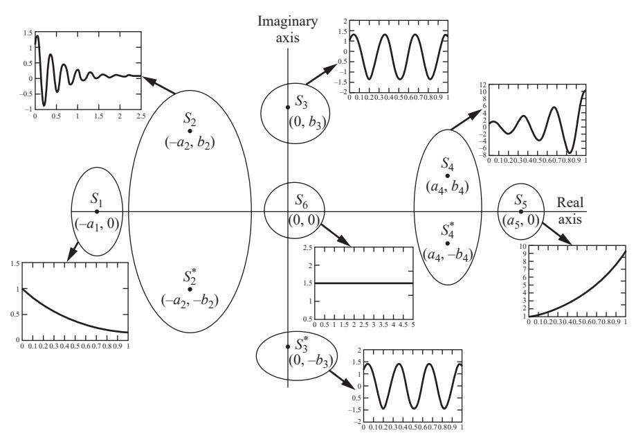
Left half-plane: decays. Right half-plane: grows. Imaginary axis: sustained oscillation. Origin: a constant.
Build on it -- one root location, one picture
- One transform per region of Fig. 3-1; invert each and plot
cases = {"real, left: 1/(s+1)": 1/(s + 1),
         "complex, left": 1/((s + 0.5)**2 + 4),
         "imaginary axis": 1/(s**2 + 4),
         "real, right: 1/(s-0.3)": 1/(s - 0.3)}
tt3 = np.linspace(0, 10, 400)
fig, axs = plt.subplots(2, 2, figsize=(7, 5.25), sharex=True)
for ax, (name, X) in zip(axs.flat, cases.items()):
    f = sp.lambdify(t, sp.inverse_laplace_transform(X, s, t))
    ax.plot(tt3, f(tt3)); ax.set_title(name, fontsize=11)
plt.tight_layout(); plt.show()

Your Turn (10 min)
Invert the Prob. 2.9 transform: $C_a(s) = \dfrac{2.5}{s(3.75s+1)} + \dfrac{11.25}{3.75s+1}$
- By hand: partial fractions and $C_a(t)$; check $t = 0$ and $t \to \infty$.
- Read the code: what does this print?
print(sp.apart(1 / (s * (s + 2)), s))
Check -- poll
Without inverting: $x(s) = \dfrac{1}{s\,(s^2 + 4)}$. For large $t$, $x(t)$ is:
A) a constant B) a constant plus a steady oscillation C) growing D) decaying to zero
Wrap-up
Derived, then coded: the mixing tee and vessel balances (Eqs. 2.1-2.4); Laplace definition and derivative rule; the three-step method (Eqs. 2.10-2.11); partial fractions for distinct, complex and repeated roots (Examples 3.1-3.5); root locations and the form of the solution.
Tools: sp.dsolve, sp.laplace_transform, sp.apart,
sp.inverse_laplace_transform, solve_ivp, sp.lambdify
Next: Ch. 4-6 -- the transfer function, first-order systems, and tanks in series.