PSE-823: Advanced Process Dynamics and Control

Lecture 2 -- Modeling and Laplace Transforms, Derived then Coded

(Coughanowr & LeBlanc, Ch. 2-3)

Date: __________

Agenda

Part A -- The mixing scenario: a mass balance becomes an ODE (Sec. 2.1)

Part B -- The heating vessel: the energy balance (Sec. 2.1)

Part C -- Laplace transforms and the three-step method (Sec. 2.2-2.3)

Part D -- Inversion by partial fractions; what the roots tell us (Ch. 3)

Same rhythm as Lecture 1: board first, then code that repeats each board step with the same step number, then code that goes further. Students read and predict; the instructor runs.

Setup (run once)

• SymPy for the algebra, NumPy/SciPy for numbers, Matplotlib to plot

import numpy as np
import matplotlib.pyplot as plt
import sympy as sp
from scipy.integrate import solve_ivp
plt.rcParams.update({"font.size": 15})
t, s = sp.symbols("t s", positive=True)

Part A

The Mixing Scenario: a Mass Balance Becomes an ODE

(Coughanowr & LeBlanc, Ch. 2, Sec. 2.1)

Introduce -- the 3:00 PM shift change (Sec. 2.1)

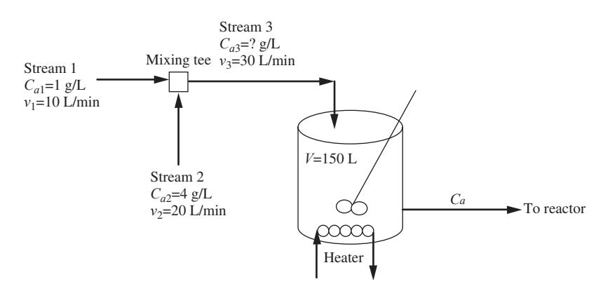
• Stream 1: 10 L/min at 1 g/L. Stream 2: 20 L/min at 4 g/L.
• They meet in a tee and feed a heating vessel ($\tau = 5$ min).
• At 3:00 PM a new operator swaps the two flow rates.
• At 3:30 PM the reactor misbehaves. What happened to the vessel's exit concentration over that half hour?

Derive 1/3 -- component balance on the tee

No holdup in a tee: rate in = rate out.

$$v_1C_{a1} + v_2C_{a2} = v_3C_{a3}$$

Before: $(10)(1) + (20)(4) = 30\,C_{a3} \Rightarrow C_{a3} = 3$ g/L. After: $(20)(1) + (10)(4) = 30\,C_{a3} \Rightarrow C_{a3} = 2$ g/L.

Derive 2/3 -- unsteady balance on the vessel

In $-$ out $=$ accumulation, constant $V$ and $v_3$:

$$v_3C_{a3} - v_3C_a = \frac{d}{dt}(VC_a) \;\Rightarrow\; \frac{V}{v_3}\frac{dC_a}{dt} + C_a = C_{a3} \qquad (2.1)$$

$\tau = V/v_3 = 5$ min (so $V = 150$ L).

Derive 3/3 -- separate and integrate

$5\,dC_a/dt + C_a = 2$ with $C_a(0) = 3$ g/L:

$$\int_3^{C_a}\frac{dC_a}{2 - C_a} = \int_0^t\frac{dt}{5} \;\Rightarrow\; C_a = 2 + e^{-t/5} \qquad (2.2)$$

Code 1/3 -- the tee balance as a function

• Mirrors Derive 1/3: solve the balance for the outlet
• Returns two values: outlet flow and outlet composition

def tee(v1, x1, v2, x2):
    v3 = v1 + v2                       # total flow
    return v3, (v1 * x1 + v2 * x2) / v3

print("before:", tee(10, 1, 20, 4))    # (30, 3.0)
print("after: ", tee(20, 1, 10, 4))    # (30, 2.0)

before: (30, 3.0)
after:  (30, 2.0)

Code walkthrough. tee takes the two flows and the two compositions and returns a tuple (v3, outlet composition). The return line is Derive 1/3 solved for C_a3. The two prints reproduce the book: (30, 3.0) before the swap and (30, 2.0) after. Note what did not change: v3 is 30 L/min in both cases, so the vessel's residence time is still 5 min. We reuse this function for temperatures in Part B -- the algebra is identical.

Code 2/3 -- the vessel balance, symbolically

• Mirrors Derive 2/3: type the balance, let SymPy rearrange it
• sp.solve(..., dC) isolates the derivative

V, v3, Ca3 = sp.symbols("V v_3 C_a3", positive=True)
Ca = sp.Function("C_a")
dC = sp.Symbol("dC")                       # stands for dC_a/dt
balance = sp.Eq(v3*Ca3 - v3*Ca(t), V*dC)   # in - out = accum.
rate = sp.solve(balance, dC)[0]
print(sp.simplify(rate))                    # v3 (C_a3 - C_a)/V
print("tau =", sp.Rational(150, 30), "min")

v_3*(C_a3 - C_a(t))/V
tau = 5 min

Code walkthrough. sp.Function("C_a") declares an unknown function so that Ca(t) can appear in equations. The derivative is held by a plain symbol dC so that sp.solve can isolate it. The balance is Derive 2/3 typed as written. The result, v3 (C_a3 - C_a)/V, is Eq. 2.1 divided by tau = V/v3. The last line evaluates tau = 150/30 = 5 min with an exact rational.

Code 3/3 -- solve the ODE with its initial condition

• Mirrors Derive 3/3: dsolve replaces separation of variables
• ics={...} supplies $C_a(0) = 3$ g/L

ode = sp.Eq(5 * Ca(t).diff(t) + Ca(t), 2)       # Eq. 2.1, numbers
Ca_t = sp.dsolve(ode, Ca(t), ics={Ca(0): 3}).rhs
print(Ca_t)                                     # Eq. 2.2
print(sp.simplify(5*Ca_t.diff(t) + Ca_t - 2))   # 0: it satisfies

2 + exp(-t/5)
0

Code walkthrough. Ca(t).diff(t) is the derivative. dsolve returns an Eq object; .rhs takes its right-hand side, the solution: 2 + exp(-t/5), Eq. 2.2. The second print substitutes the answer back into the ODE and simplifies the residual to 0 -- the check the book asks the reader to do by hand ("Eq. 3.6 by substitution into the original differential equation").

Build on it -- a numerical solution that knows no calculus

• solve_ivp integrates the ODE step by step from $C_a(0)$
• Compare with Eq. 2.2 at every point

def vessel(t, C, Cin):
    return [(Cin - C[0]) / 5.0]        # Eq. 2.1: dC/dt

tt = np.linspace(0, 30, 61)            # 3:00 to 3:30 PM
num = solve_ivp(vessel, [0, 30], [3.0], args=(2.0,),
                t_eval=tt, rtol=1e-8).y[0]
exact = 2 + np.exp(-tt / 5)            # Eq. 2.2
print(f"max |numerical - exact| = {np.abs(num - exact).max():.1e}")
print(f"C_a at 3:30 PM = {num[-1]:.4f} g/L")

max |numerical - exact| = 2.5e-07
C_a at 3:30 PM = 2.0025 g/L

Code walkthrough. vessel returns dC/dt from Eq. 2.1; args=(2.0,) passes the new inlet concentration. solve_ivp advances the solution in small steps; t_eval asks for 61 output times over the half hour, and rtol=1e-8 tightens the accuracy. The first print compares with the exact Eq. 2.2: the gap is a few times 1e-7 g/L. The second answers the book's question: at 3:30 PM the exit concentration is 2.0025 g/L -- the vessel has essentially finished its transition (six time constants).

Plot -- the operator-induced transient (cf. Fig. 2-3)

• Exact solution as a line, numerical solution as dots

fig, ax = plt.subplots(figsize=(7, 5.25))
ax.plot(tt, exact, label="Eq. 2.2, exact")
ax.plot(tt[::4], num[::4], "o", label="solve_ivp")
ax.axhline(2, ls="--", c="gray")
ax.set(xlabel="minutes after 3:00 PM", ylabel="C_a (g/L)")
ax.legend(loc="upper right")
plt.show()

Code walkthrough. tt[::4] takes every fourth point so the dots do not crowd the line. The curve starts at 3 g/L and decays toward the dashed 2 g/L line with time constant 5 min: 63% of the drop by 3:05, 95% by 3:15. Line and dots coincide: two independent routes to the same answer.

Your Turn (10 min)

Prob. 2.9. Instead, at 3:00 PM the operator increases stream 1 to 20 L/min; stream 2 (20 L/min, 4 g/L) is unchanged; $V = 150$ L.

1. By hand: the new $v_3$, $C_{a3}$ and $\tau$.
2. Read the code: what does this print?

v3, Ca3 = tee(20, 1, 20, 4)
print(v3, Ca3, 150 / v3)

(1) v3 = 40 L/min; Ca3 = (20 + 80)/40 = 2.5 g/L; tau = 150/40 = 3.75 min. (2) Prints 40 2.5 3.75. Common slip: keeping tau = 5 min. This time v3 changed, so the residence time changed too.

Check -- cold-call

In the book's swap, $\tau$ stayed at 5 min. In Prob. 2.9 it fell to 3.75 min. Which single quantity decides whether $\tau$ changes?

v3, the total throughput: tau = V/v3. The swap kept v1 + v2 = 30, so only the inlet composition changed (a disturbance in the forcing). In Prob. 2.9 the flow itself changed, so the process dynamics changed.

Part B

The Heating Vessel: the Energy Balance

(Coughanowr & LeBlanc, Ch. 2, Sec. 2.1)

Introduce -- the same scenario, now for temperature

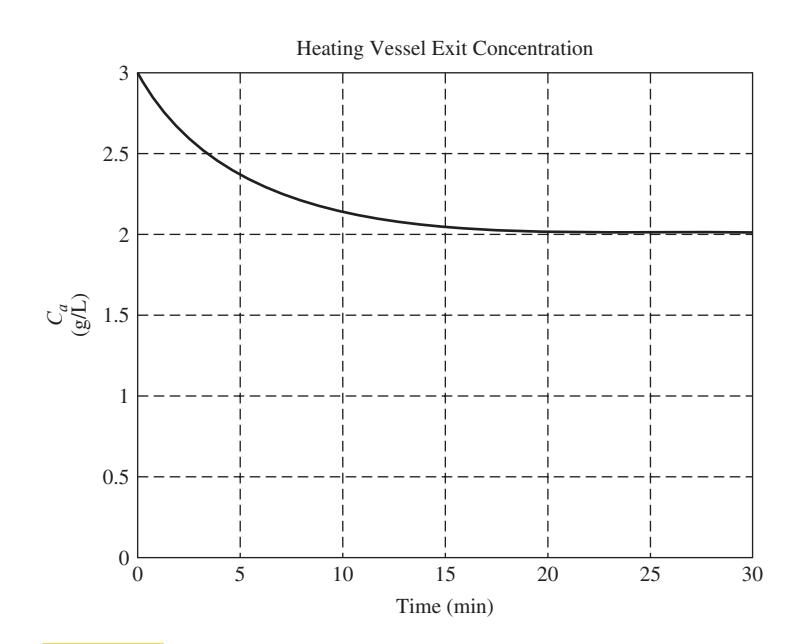
• Stream 1 at 25 C, stream 2 at 55 C. The heater brings the vessel outlet to 80 C.
• After the swap, with the heater unchanged: what does the reactor feed temperature do?

Derive 1/3 -- energy balance on the tee

Constant $\rho$ and $C_p$; enthalpy relative to $T_{ref}$:

$$v_1T_1 + v_2T_2 = v_3T_3 \;\Rightarrow\; T_3 = \frac{(10)(25) + (20)(55)}{30} = 45\ ^\circ\text{C}$$

After the swap: $T_3 = [(20)(25) + (10)(55)]/30 = 35$ C.

Derive 2/3 -- the heater duty at steady state

Vessel: in + heat = out:

$$Q = \rho v_3C_p(T - T_3) = (1000)(30)(1)(80 - 45) = 1.05\times10^6\ \text{cal/min} = 73.2\ \text{kW}$$

Derive 3/3 -- unsteady energy balance

Add accumulation $\frac{d}{dt}[\rho VC_p(T - T_{ref})]$ and divide by $\rho v_3 C_p$:

$$\tau\frac{dT}{dt} + T = T_3 + \frac{Q}{\rho v_3C_p} \qquad (2.3)$$

$5\,dT/dt + T = 35 + 35 = 70$, $T(0) = 80$: $\;T = 70 + 10e^{-t/5}$ (2.4).

Code 1/3 -- the tee function again, for temperatures

• Mirrors Derive 1/3: same balance, temperatures instead of $C$
• No new code: the algebra is identical

print("T3 before:", tee(10, 25, 20, 55)[1], "C")
print("T3 after: ", tee(20, 25, 10, 55)[1], "C")

T3 before: 45.0 C
T3 after:  35.0 C

Code walkthrough. tee(...)[1] takes the second element of the returned tuple, the outlet composition -- here the outlet temperature. Prints 45.0 C and 35.0 C. The point: the energy balance on the tee (constant rho and Cp) has the same form as the component balance, so the same function serves both.

Code 2/3 -- heater duty, with units

• Mirrors Derive 2/3; then convert cal/min to kW
• 1 cal = 4.184 J; 1 min = 60 s

rho, Cp, v3n = 1000.0, 1.0, 30.0      # g/L, cal/(g C), L/min
Q = rho * v3n * Cp * (80 - 45)        # cal/min
print(f"Q = {Q:.3g} cal/min = {Q * 4.184 / 60 / 1000:.1f} kW")

Q = 1.05e+06 cal/min = 73.2 kW

Code walkthrough. The first line sets the book's constants. Line 2 is Derive 2/3. The f-string formats Q with three significant figures (.3g) and converts: cal/min times 4.184 J/cal divided by 60 s/min gives W, then /1000 for kW. Prints Q = 1.05e+06 cal/min = 73.2 kW, the book's numbers.

Code 3/3 -- solve Eq. 2.3 after the swap

• Mirrors Derive 3/3: dsolve with $T(0) = 80$ C

T = sp.Function("T")
heat = sp.Rational(35)                     # Q/(rho v3 Cp), C
ode_T = sp.Eq(5 * T(t).diff(t) + T(t), 35 + heat)
T_t = sp.dsolve(ode_T, T(t), ics={T(0): 80}).rhs
print(T_t)                                 # Eq. 2.4

70 + 10*exp(-t/5)

Code walkthrough. Q/(rho v3 Cp) = 1.05e6/30000 = 35 C: the temperature rise the heater supplies. The ODE is Eq. 2.3 with T3 = 35 C after the swap. dsolve returns 70 + 10 exp(-t/5): Eq. 2.4. Same shape as Eq. 2.2, because Eq. 2.1 and Eq. 2.3 are the same first-order equation with the same tau.

Build on it -- what heater duty restores 80 C?

• Steady state: $Q = \rho v_3 C_p (80 - T_3)$ with $T_3 = 35$ C
• Simulate: the heater is raised at $t = 10$ min

Q_new = rho * v3n * Cp * (80 - 35)           # cal/min
def heater(t, T, Q_of_t):
    return [(35 - T[0] + Q_of_t(t) / (rho*v3n*Cp)) / 5]
Q_sched = lambda t: Q if t < 10 else Q_new   # raise at 10 min
tt2 = np.linspace(0, 40, 401)
T_sim = solve_ivp(heater, [0, 40], [80.0], args=(Q_sched,),
                  t_eval=tt2, max_step=0.1).y[0]
print(f"Q_new = {Q_new:.3g} cal/min = "
      f"{Q_new * 4.184 / 60000:.1f} kW; T(40) = {T_sim[-1]:.2f} C")

Q_new = 1.35e+06 cal/min = 94.1 kW; T(40) = 79.98 C

Code walkthrough. The steady-state duty needed for 80 C with a 35 C feed is rho v3 Cp (80 - 35) = 1.35e6 cal/min (94.1 kW). heater is Eq. 2.3 with Q supplied by a function of time, Q_sched: a lambda that returns the old duty before 10 min and the new duty after. max_step=0.1 stops the solver stepping over the switch. T(40) prints 79.98 C: the outlet falls toward 70 C for ten minutes, then recovers to 80 C. Raising Q by the right amount at the right time is exactly the job a temperature controller will do (Lecture 4 onward).

Plot -- disturbance, then a manual correction

• The feed cools at $t = 0$; the heater is raised at $t = 10$

fig, ax = plt.subplots(figsize=(7, 5.25))
ax.plot(tt2, T_sim)
ax.plot(tt2, 70 + 10 * np.exp(-tt2 / 5), "--",
        label="no correction (Eq. 2.4)")
ax.axvline(10, ls=":", c="k")
ax.set(xlabel="minutes after 3:00 PM", ylabel="T (C)")
ax.legend(loc="lower right")
plt.show()

Code walkthrough. Solid: the simulated outlet. Dashed: Eq. 2.4, what happens if nobody acts. They coincide until the dotted line at 10 min; then the solid curve turns and climbs back to 80 C with the same 5-min time constant. The deviation peaked at 8.6 C below set point: the cost of a 10-minute reaction time.

Your Turn (8 min)

Prob. 2.9, energy part: stream 1 rises to 20 L/min at 25 C, stream 2 stays 20 L/min at 55 C, $Q = 1.05\times10^6$ cal/min.

1. By hand: the new $T_3$, $\tau$, and final outlet temperature.
2. Read the code: what does this print?

print(tee(20, 25, 20, 55)[1] + 1.05e6 / (1000 * 40))

(1) T3 = (500 + 1100)/40 = 40 C; tau = 150/40 = 3.75 min; final T = T3 + Q/(rho v3 Cp) = 40 + 1.05e6/40000 = 40 + 26.25 = 66.25 C. (2) Prints 66.25: the same calculation. Slip: dividing Q by the old 30000 (rho v3 Cp with v3 = 30) and getting 75 C.

Check -- think-pair-share

The concentration and the temperature responses have exactly the same shape. Is that a coincidence of the numbers, or does it follow from Eq. 2.1 and Eq. 2.3? What would make them differ?

It follows from the equations: both are first order with the same tau = V/v3 and both are driven by a step. They would differ if the vessel had heat capacity in its walls (an extra lag for T only), heat loss, or a reaction that consumes A.

Part C

Laplace Transforms and the Three-Step Method

(Coughanowr & LeBlanc, Ch. 2, Sec. 2.2-2.3)

Introduce -- why transform at all?

• Separation of variables worked once. Higher-order models will not separate.
• The Laplace transform turns differentiation into multiplication by $s$ -- an ODE becomes algebra.
• Definition (Eq. 2.5): $F(s) = \int_0^\infty f(t)\,e^{-st}\,dt$

Derive 1/3 -- the transform of a step (Ex. 2.1)

Apply the definition to $f(t) = 1$:

$$F(s) = \int_0^\infty e^{-st}dt = -\frac{e^{-st}}{s}\Big|_0^\infty = \frac{1}{s}$$

Derive 2/3 -- the transform of a derivative

Integrate by parts, $u = e^{-st}$, $dv = f'\,dt$:

$$\mathcal{L}\left\{\frac{df}{dt}\right\} = sF(s) - f(0) \qquad (2.6)$$

The initial condition enters here, and only here.

Derive 3/3 -- transform the mixing balance

$5\,dC_a/dt + C_a = 2$, $C_a(0) = 3$:

$$5[sC_a(s) - 3] + C_a(s) = \frac{2}{s} \;\Rightarrow\; C_a(s) = \frac{2}{s(5s+1)} + \frac{15}{5s+1} \qquad (2.10)$$

Code 1/3 -- the definition, then the table

• Mirrors Derive 1/3: sp.integrate the definition directly
• Then sp.laplace_transform reproduces Table 2.1 entries

a, k = sp.symbols("a k", positive=True)
print(sp.integrate(sp.exp(-s * t), (t, 0, sp.oo)))   # 1/s
for f in [sp.exp(-a * t), t, sp.sin(k * t), sp.cos(k * t)]:
    F = sp.laplace_transform(f, t, s, noconds=True)
    print(f, "->", F)

1/s

exp(-a*t) -> 1/(a + s)
t -> s**(-2)
sin(k*t) -> k/(k**2 + s**2)
cos(k*t) -> s/(k**2 + s**2)

Code walkthrough. Line 2 evaluates the defining integral of Eq. 2.5 for f = 1; sp.oo is infinity. It prints 1/s, Ex. 2.1. The loop transforms four table entries; noconds=True drops the convergence conditions (Re s > -a, and so on). Expected: exp(-a t) -> 1/(a + s), t -> 1/s2, sin(k t) -> k/(k2 + s2), cos(k t) -> s/(k2 + s**2). These are rows of Table 2.1.

Code 2/3 -- the derivative rule, checked

• Mirrors Derive 2/3 on a concrete function
• Left: transform of $f'$. Right: $sF(s) - f(0)$

f = 3 * sp.exp(-2 * t) + t                  # any test function
lhs = sp.laplace_transform(f.diff(t), t, s, noconds=True)
F = sp.laplace_transform(f, t, s, noconds=True)
rhs = s * F - f.subs(t, 0)                  # Eq. 2.6
print(sp.simplify(lhs - rhs))               # 0

0

Code walkthrough. A test function with f(0) = 3 is chosen so the f(0) term matters. lhs transforms the derivative directly; rhs builds s F(s) - f(0) from Eq. 2.6 (f.subs(t, 0) evaluates f at t = 0). Their difference simplifies to 0. One example is not a proof -- the board derivation is the proof -- but it catches a sign error at once.

Code 3/3 -- the three-step method, step 2

• Mirrors Derive 3/3: transform each side, solve for $C_a(s)$
• The symbol Cs stands for $C_a(s)$

Cs = sp.Symbol("C_s")
step1 = sp.Eq(5 * (s * Cs - 3) + Cs, 2 / s)   # Eq. 2.6 used
Ca_s = sp.solve(step1, Cs)[0]
print(sp.apart(Ca_s, s))
print(sp.simplify(Ca_s - (2/(s*(5*s+1)) + 15/(5*s+1))))

5/(5*s + 1) + 2/s
0

Code walkthrough. Step 1 is typed with the derivative rule already applied: 5[s C - 3] + C = 2/s. sp.solve performs step 2, isolating C_s. The first print shows apart's split of the result (a preview of Part D): 2/s + 5/(5 s + 1). The second print confirms the result equals the book's Eq. 2.10 term by term: 0.

Build on it -- Example 2.2, third order

• A third-order ODE, all initial conditions zero
• By hand: three derivative transforms. Here: one line each

x = sp.Function("x")
ode3 = sp.Eq(x(t).diff(t, 3) + 4*x(t).diff(t, 2)
             + 5*x(t).diff(t) + 2*x(t), 2)
x_t = sp.dsolve(ode3, x(t), ics={x(0): 0, x(t).diff(t).subs(t, 0): 0,
                                 x(t).diff(t, 2).subs(t, 0): 0}).rhs
print(sp.expand(x_t))                          # Eq. 2.8
print(sp.apart(sp.laplace_transform(x_t, t, s, noconds=True), s))

-2*t*exp(-t) + 1 - exp(-2*t)
-1/(s + 2) - 2/(s + 1)**2 + 1/s

Code walkthrough. x(t).diff(t, 3) is the third derivative. The ics dictionary sets x(0), x'(0) and x''(0) to zero; derivatives at 0 are written as x(t).diff(t).subs(t, 0). dsolve returns Eq. 2.8: 1 - 2 t exp(-t) - exp(-2 t). Transforming it back and applying apart gives Eq. 2.9: 1/s - 2/(s + 1)**2 - 1/(s + 2). Getting from Eq. 2.7 to Eq. 2.9 by hand is the subject of Part D.

Your Turn (8 min)

Ex. 2.4. Solve $dx/dt + 3x = 0$, $x(0) = 2$, by the three steps.

1. By hand: $x(s)$, then $x(t)$.
2. Read the code: what does this print?

print(sp.laplace_transform(t**2, t, s, noconds=True))

(1) [s x(s) - 2] + 3 x(s) = 0, so x(s) = 2/(s + 3) and x(t) = 2 e^(-3t). (2) Prints 2/s3 (Table 2.1: t^n -> n!/s^(n+1)). Slip: 1/s3.

Check -- cold-call

In the three-step method, at which step do the initial conditions enter -- and what does that imply about the form of the solution?

Step 1, through Eq. 2.6 (and only there). They change the numerator of x(s), never the denominator, so they change the coefficients of the solution's terms but not which terms (exponentials, sines) appear.

Part D

Inversion by Partial Fractions; What the Roots Tell Us

(Coughanowr & LeBlanc, Ch. 3, Sec. 3.1-3.2)

Introduce -- the third step: back to the time domain

• $x(s)$ rarely appears in Table 2.1 as it stands.
• Split it into simple fractions that do: partial fractions.
• Distinct real roots: Heaviside cover-up. Complex roots: keep the quadratic, complete the square. Repeated roots: match coefficients.

Derive 1/4 -- Ex. 3.1, the cover-up rule

$dx/dt + x = 1$, $x(0) = 0$ gives $x(s) = 1/[s(s+1)]$:

$$\frac{1}{s(s+1)} = \frac{A}{s} + \frac{B}{s+1}: \quad A = \frac{1}{0+1} = 1,\;\; B = \frac{1}{-1} = -1$$

$$x(t) = 1 - e^{-t} \qquad (3.6)$$

Derive 2/4 -- Ex. 3.2, the mixing scenario inverted

Eq. 2.10, with $5s + 1 = 5(s + \frac15)$:

$$C_a(s) = \frac{2}{s} - \frac{2}{s+\frac15} + \frac{3}{s+\frac15} = \frac{2}{s} + \frac{1}{s+\frac15} \;\Rightarrow\; C_a(t) = 2 + e^{-t/5}$$

The same answer as Part A, by a different road.

Derive 3/4 -- Ex. 3.4, complex roots

$x'' + 2x' + 2x = 2$, zero ICs: $x(s) = 2/[s(s^2+2s+2)]$, roots $-1 \pm j$:

$$x(s) = \frac{1}{s} - \frac{(s+1) + 1}{(s+1)^2 + 1^2} \;\Rightarrow\; x(t) = 1 - e^{-t}(\cos t + \sin t)$$

Derive 4/4 -- Ex. 3.5, a repeated root

$x(s) = 1/[s(s+1)^3]$: cover-up gives $A = 1$, $B = -1$; matching coefficients gives $C = D = -1$:

$$x(t) = 1 - e^{-t}\left(\frac{t^2}{2} + t + 1\right) \qquad (3.17)$$

Code 1/4 -- Ex. 3.1: apart is the cover-up rule

• Mirrors Derive 1/4: split, then invert
• inverse_laplace_transform replaces the table lookup

X1 = 1 / (s * (s + 1))
print(sp.apart(X1, s))                          # 1/s - 1/(s + 1)
print(sp.inverse_laplace_transform(X1, s, t))   # 1 - exp(-t)

-1/(s + 1) + 1/s
1 - exp(-t)

Code walkthrough. sp.apart(X1, s) returns the partial-fraction expansion in s: the A = 1 and B = -1 found by cover-up. inverse_laplace_transform goes straight to the time domain: 1 - exp(-t), Eq. 3.6. (SymPy may print the second line with a Heaviside(t) factor in some versions; for t > 0 it is 1.)

Code 2/4 -- Ex. 3.2: the scenario, inverted

• Mirrors Derive 2/4 with the transform from Part C

print(sp.apart(Ca_s, s))
print(sp.inverse_laplace_transform(Ca_s, s, t))
T_s = 70 / (s * (5*s + 1)) + 400 / (5*s + 1)     # Eq. 2.11
print(sp.inverse_laplace_transform(T_s, s, t))

5/(5*s + 1) + 2/s
2 + exp(-t/5)
70 + 10*exp(-t/5)

Code walkthrough. Ca_s is the C_a(s) solved in Part C (Eq. 2.10). apart returns 2/s + 5/(5 s + 1), which is 2/s + 1/(s + 1/5): Derive 2/4. Inverting gives 2 + exp(-t/5), the answer of Part A. The last two lines invert Eq. 2.11 to 70 + 10 exp(-t/5), the answer of Part B. Three routes -- separation, dsolve, Laplace -- now agree for both balances.

Code 3/4 -- Ex. 3.4: complex roots

• Mirrors Derive 3/4; apart keeps the quadratic unfactored
• sp.roots shows the complex pair

X4 = 2 / (s * (s**2 + 2*s + 2))
print(sp.roots(s**2 + 2*s + 2))                 # -1 +/- I
print(sp.apart(X4, s))                          # 1/s - (s+2)/(...)
x4 = sp.inverse_laplace_transform(X4, s, t)
print(sp.simplify(x4))

{-1 - I: 1, -1 + I: 1}
-(s + 2)/(s**2 + 2*s + 2) + 1/s
1 - sqrt(2)*exp(-t)*sin(t + pi/4)

Code walkthrough. sp.roots returns a dictionary root -> multiplicity: {-1 - I: 1, -1 + I: 1} (I is sqrt(-1)). apart returns 1/s - (s + 2)/(s**2 + 2 s + 2): the B = -1, C = -2 of the book's coefficient matching, with the quadratic left intact, exactly the method of Ex. 3.4. The inverse simplifies to the book's 1 - exp(-t)(sin t + cos t), possibly written as 1 - sqrt(2) exp(-t) sin(t + pi/4) -- the same function.

Code 4/4 -- Ex. 3.5 and Ex. 3.3

• Mirrors Derive 4/4: repeated roots, no special handling
• Then Ex. 3.3: five distinct roots, one line

X5 = 1 / (s * (s + 1)**3)
print(sp.apart(X5, s))
X3 = (s**4 - 6*s**2 + 9*s - 8) / (s*(s-2)*(s+1)*(s+2)*(s-1))
print(sp.apart(X3, s))

-1/(s + 1) - 1/(s + 1)**2 - 1/(s + 1)**3 + 1/s
-17/(12*(s + 2)) + 11/(3*(s + 1)) + 2/(3*(s - 1)) + 1/(12*(s - 2)) - 2/s

Code walkthrough. For Ex. 3.5, apart returns 1/s - 1/(s + 1) - 1/(s + 1)**2 - 1/(s + 1)**3: A = 1, B = C = D = -1, Eq. 3.16, with no separate procedure for the repeated root. For Ex. 3.3 it returns the five coefficients the book tabulates: -2/s + 1/(12 (s - 2)) + 11/(3 (s + 1))

• 17/(12 (s + 2)) + 2/(3 (s - 1)). The book needs MATLAB's diff(int()) trick for this; SymPy has a dedicated function.

Introduce -- the form of $x(t)$ without inverting (Sec. 3.2)

Each root of the denominator of $x(s)$ contributes one kind of term:

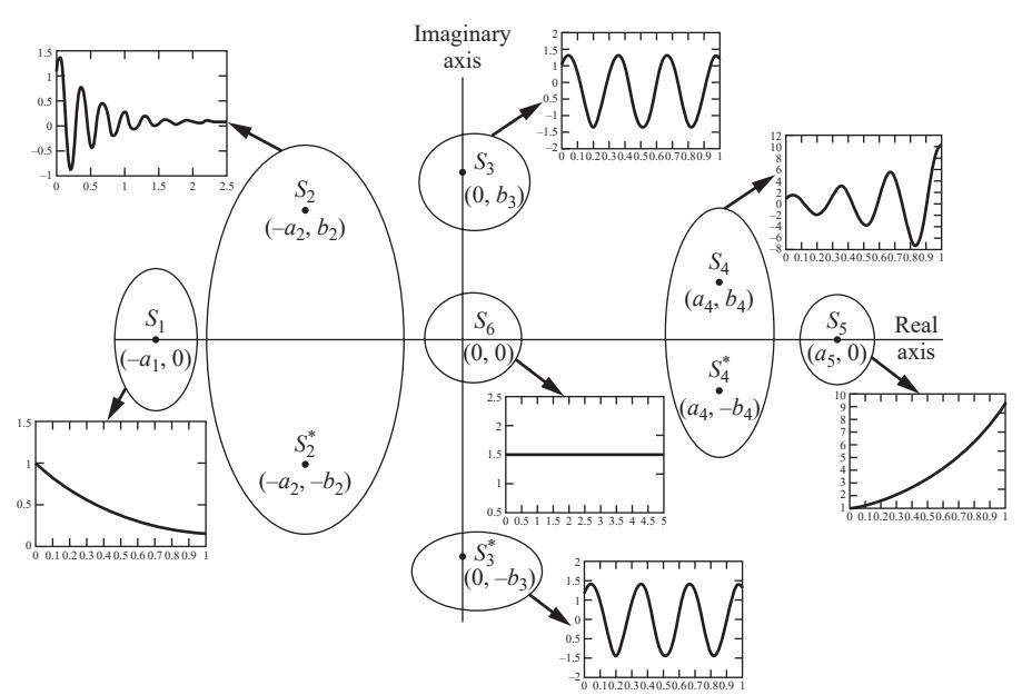
Left half-plane: decays. Right half-plane: grows. Imaginary axis: sustained oscillation. Origin: a constant.

Build on it -- one root location, one picture

• One transform per region of Fig. 3-1; invert each and plot

cases = {"real, left: 1/(s+1)": 1/(s + 1),
         "complex, left": 1/((s + 0.5)**2 + 4),
         "imaginary axis": 1/(s**2 + 4),
         "real, right: 1/(s-0.3)": 1/(s - 0.3)}
tt3 = np.linspace(0, 10, 400)
fig, axs = plt.subplots(2, 2, figsize=(7, 5.25), sharex=True)
for ax, (name, X) in zip(axs.flat, cases.items()):
    f = sp.lambdify(t, sp.inverse_laplace_transform(X, s, t))
    ax.plot(tt3, f(tt3)); ax.set_title(name, fontsize=11)
plt.tight_layout(); plt.show()

Code walkthrough. cases maps a label to a transform with one root (or one complex pair) in each region of Fig. 3-1. For each, SymPy inverts the transform and sp.lambdify turns the formula into a NumPy function that can be evaluated on the time grid. zip(axs.flat, ...) pairs each of the four panels with one case. Read the panels against Table 3.1: a decaying exponential; a decaying oscillation (roots -0.5 +/- 2j); a sustained sine (roots +/- 2j); an exponential that grows without bound (root +0.3). Stability, in Lecture 6, is the question "are all roots in the left half-plane?"

Your Turn (10 min)

Invert the Prob. 2.9 transform: $C_a(s) = \dfrac{2.5}{s(3.75s+1)} + \dfrac{11.25}{3.75s+1}$

1. By hand: partial fractions and $C_a(t)$; check $t = 0$ and $t \to \infty$.
2. Read the code: what does this print?

print(sp.apart(1 / (s * (s + 2)), s))

(1) 3.75 s + 1 = 3.75 (s + 0.2667). First term: A/s + B/(s + 0.2667) with A = 2.5, B = -2.5. Second term: 3/(s + 0.2667). Sum: 2.5/s + 0.5/(s + 0.2667), so C_a(t) = 2.5 + 0.5 e^(-t/3.75). Checks: C_a(0) = 3 (the old steady state), C_a(inf) = 2.5 (the new). (2) -1/(2*(s + 2)) + 1/(2*s). Slip: forgetting to divide by 2 at the cover-up (A = 1/(0 + 2) = 1/2).

Check -- poll

Without inverting: $x(s) = \dfrac{1}{s\,(s^2 + 4)}$. For large $t$, $x(t)$ is:

A) a constant B) a constant plus a steady oscillation C) growing D) decaying to zero

B. The root at s = 0 gives a constant; the roots +/- 2j on the imaginary axis give an undamped oscillation of frequency 2. Exactly: x(t) = (1 - cos 2t)/4. The bottom-left panel of the gallery.

Wrap-up

Derived, then coded: the mixing tee and vessel balances (Eqs. 2.1-2.4); Laplace definition and derivative rule; the three-step method (Eqs. 2.10-2.11); partial fractions for distinct, complex and repeated roots (Examples 3.1-3.5); root locations and the form of the solution.

Tools: sp.dsolve, sp.laplace_transform, sp.apart, sp.inverse_laplace_transform, solve_ivp, sp.lambdify

Next: Ch. 4-6 -- the transfer function, first-order systems, and tanks in series.