How every lecture works
- Each idea is introduced as a physical question.
- It is derived on the board, one step per slide.
- Then code repeats the derivation, step for step.
- Then the code goes further than hand algebra can.
- In class you read the code and predict what it prints.
The course in one picture
- Coughanowr & LeBlanc -- the spine (about 80%): models, transfer functions, stability, frequency response, state space.
- Cecil Smith -- the industrial layer (about 20%): cascade, override, ratio, decoupling, and the course's only MPC source.
- Weeks 1-8: classical theory, then the midterm.
- Weeks 9-15: advanced strategies, identification, MPC.
Agenda
Part A -- Feedback control of a hot water tank (Ch. 1, Ex. 1.1)
Part B -- Proportional and integral control; offset (Ch. 1)
Part C -- Apparent error and a first look at instability (Ch. 1)
Part D -- Narrow the variance, shift the target; DCS blocks (Cecil Smith, Intro and Sec. 1.1-1.2)
Setup (run once)
- Every library this lecture uses, imported once
plt.rcParamsmakes plot text readable on the projector
import numpy as np
import matplotlib.pyplot as plt
import sympy as sp
plt.rcParams.update({"font.size": 15})
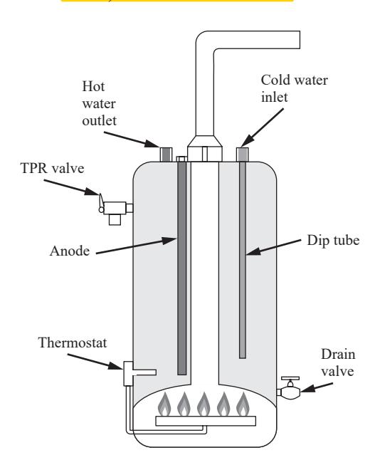
Introduce -- the home hot water heater (Ex. 1.1)
- Controlled variable: water temperature $T$; set point 130 F.
- Manipulated variable: fuel to the burner (valve open or shut).
- Disturbances: hot water drawn off and replaced by cold feed; heat lost to the surroundings.
- Thermocouple measures $T$; the thermostat is the controller.
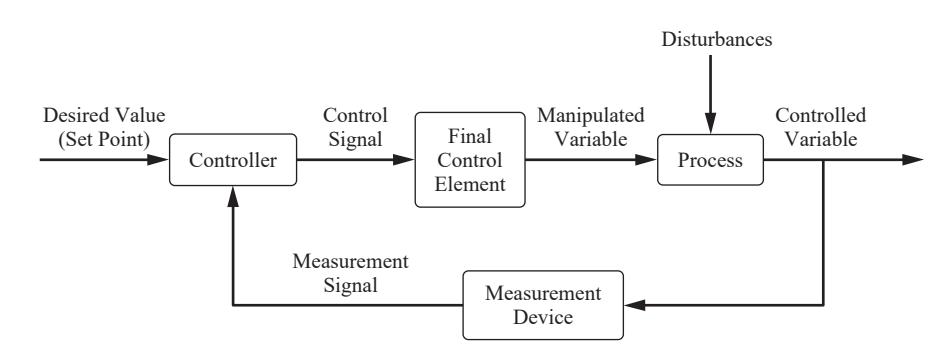
Introduce -- the block diagram (Fig. 1-1, Fig. 1-3)
Information flows around a loop: measure, compare, act.
Introduce -- a model to experiment with
To simulate the tank we need its dynamics. Lecture 2 derives them from an energy balance; for now we take the result:
$$\tau\,\frac{dT}{dt} = (T_i - T) + K\,q$$
$T_i$: cold feed temperature, $q$: burner on-fraction (0 to 1). Illustrative values: $\tau = 30$ min, $K = 90$ F, $T_i = 60$ F.
Derive 1/2 -- the error and the on/off law
The thermostat computes the error (Ch. 1):
$$e = T_{\text{set}} - T_{\text{measured}}$$
On/off law: if $e > 0$ open the fuel valve ($q=1$); if $e \le 0$ close it ($q=0$). No values in between.
Derive 2/2 -- what burner fraction does 130 F need?
At steady state $dT/dt = 0$, so $0 = (T_i - T) + Kq$:
$$q_s = \frac{T - T_i}{K} = \frac{130 - 60}{90} = 0.778$$
On/off cannot output 0.778. It must cycle: on about 78% of the time, off about 22%.
Code 1/3 -- the tank model as a function
- A Python
defturns the model equation into reusable code - It returns $dT/dt$: the right-hand side divided by $\tau$
- Mirrors the model slide, symbol for symbol
tau, K = 30.0, 90.0                 # min, F

def dTdt(T, Ti, q):
    # tau dT/dt = (Ti - T) + K q
    return ((Ti - T) + K * q) / tau

print(dTdt(130.0, 60.0, 0.778))     # ~0 at steady state
print(dTdt(130.0, 60.0, 1.0))       # burner on: heating
0.000666666666666534
0.6666666666666666
Code 2/3 -- the thermostat as a function
- The on/off law of Derive 1/2, in four lines
if ... elseis the decision; there is no middle value
def thermostat(T_meas, T_set=130.0):
    e = T_set - T_meas          # error (Ch. 1)
    return 1.0 if e > 0 else 0.0

for T in [128.0, 130.0, 131.5]:
    print(T, "->", thermostat(T))
128.0 -> 1.0
130.0 -> 0.0
131.5 -> 0.0
Code 3/3 -- closing the loop, one sample at a time
- Every
dtminutes: measure, decide, update the tank - The update is Euler's method: $T \leftarrow T + \Delta t\,dT/dt$
- Start cold (100 F) and run for 90 min
dt, T = 0.1, 100.0               # min, F (cold start)
log_T, log_q = [], []
for k in range(int(90 / dt)):
    q = thermostat(T)            # measure and decide
    T = T + dt * dTdt(T, 60.0, q)  # tank responds
    log_T.append(T)
    log_q.append(q)
log_T, log_q = np.array(log_T), np.array(log_q)
i = np.argmax(log_T >= 130)      # first time at set point
print(f"reaches 130 F at {i*dt:.1f} min")
print(f"burner on {log_q[i:].mean():.1%} of the time after")
reaches 130 F at 27.4 min
burner on 77.6% of the time after
Plot -- on/off control in action
- Top: temperature. Bottom: burner state
sharex=Truelines the two time axes up
t = np.arange(len(log_T)) * dt
fig, (ax1, ax2) = plt.subplots(2, 1, figsize=(7, 5.25),
                               sharex=True)
ax1.plot(t, log_T)
ax1.axhline(130, ls="--", c="gray")
ax1.set_ylabel("T (F)")
ax2.step(t, log_q, where="post")
ax2.set(xlabel="t (min)", ylabel="burner")
plt.show()

Your Turn (8 min)
- By hand: in winter the cold feed drops to $T_i = 50$ F. What fraction of the time must the burner now be on?
- Read the code: what does this print?
for T in [131.0, 129.9]:
    print(thermostat(T, T_set=132.0))
Check -- cold-call
The thermocouple wire breaks and the thermostat stops receiving $T$.
Is this still a control system? Which word in Ch. 1 describes it?
Introduce -- act in proportion to the error
- Proportional (P): change the heat input in proportion to $e$: $$q = q_s + K_c\,e$$
- $K_c$ is the controller gain, our design choice.
- Book's claim: larger $K_c$, smaller steady error -- but never zero.
- Test case: winter arrives, $T_i$ drops from 60 to 50 F.
Derive 1/3 -- steady state with the P law
Set $dT/dt = 0$ and substitute the controller:
$$0 = (T_i - T) + K\left[q_s + K_c\,(T_{set} - T)\right]$$
Derive 2/3 -- deviation variables
Subtract the old steady state; let $T' = T - T_{set}$, $T_i' = T_i - 60$:
$$0 = T_i' - T' - K K_c\,T' \;\Rightarrow\; T' = \frac{T_i'}{1 + K K_c}$$
Derive 3/3 -- the offset
Offset is the steady-state error, $e_{ss} = -T'$:
$$e_{ss} = \frac{-T_i'}{1 + K K_c} = \frac{10}{1 + 90 K_c}\ \text{F}$$
Finite for every finite $K_c$: proportional control always leaves an offset. Integral action adds $\frac{K_c}{\tau_I}\int e\,dt$, which can only stop changing when $e = 0$.
Code 1/3 -- the steady-state balance, symbolically
- Mirrors Derive 1/3 and 2/3: same equation, typed as written
sp.symbolsdeclares the letters;sp.solveisolates $T'$
Tp, Tip, K_, Kc = sp.symbols("T' T_i' K K_c")
balance = sp.Eq(0, Tip - Tp - K_ * Kc * Tp)   # Derive 2/3
T_ss = sp.solve(balance, Tp)[0]
T_ss
Code 2/3 -- offset for several gains
- Offset $e_{ss} = -T'$; substitute $T_i' = -10$ F and $K = 90$ F
subsreplaces symbols with numbers;floatgives a decimal
e_ss = -T_ss.subs({Tip: -10, K_: 90})        # Derive 3/3
for kc in [0.01, 0.05, 0.1, 0.5]:            # 1/F
    print(f"Kc = {kc:4}: offset = {float(e_ss.subs(Kc, kc)):.2f} F")
Kc = 0.01: offset = 5.26 F
Kc = 0.05: offset = 1.82 F
Kc =  0.1: offset = 1.00 F
Kc =  0.5: offset = 0.22 F
Code 3/3 -- the limit of infinite gain
sp.limitasks what happens as $K_c \to \infty$- The answer is zero -- reached only in the limit
print(sp.limit(e_ss, Kc, sp.oo))        # 0
print(sp.solve(sp.Eq(e_ss, 0), Kc))     # no finite Kc
0
[]
Build on it -- simulate P and PI after the disturbance
- The Part A loop again, with a P or PI law instead of on/off
- Disturbance: $T_i$ steps 60 to 50 F at $t = 10$ min
np.clipkeeps the burner between 0 and 1
def run(Kc, tauI=None, t_end=150.0, dt=0.1):
    T, I, out = 130.0, 0.0, []
    for k in range(int(t_end / dt)):
        Ti = 60.0 if k * dt < 10 else 50.0
        e = 130.0 - T
        I += e * dt                          # integral of error
        q = 70/90 + Kc * (e + (I / tauI if tauI else 0))
        T += dt * dTdt(T, Ti, np.clip(q, 0, 1))
        out.append(T)
    return np.array(out)
T_P, T_PI = run(0.05), run(0.05, tauI=10.0)
print(f"P: {T_P[-1]:.2f} F   PI: {T_PI[-1]:.2f} F")
P: 128.18 F PI: 130.00 F
Plot -- P leaves an offset, PI removes it
- Same disturbance, same gain; only the integral term differs
t = np.arange(len(T_P)) * 0.1
fig, ax = plt.subplots(figsize=(7, 5.25))
ax.plot(t, T_P, label="P, Kc = 0.05")
ax.plot(t, T_PI, label="PI, tau_I = 10 min")
ax.axhline(130, ls="--", c="gray")
ax.set(xlabel="t (min)", ylabel="T (F)")
ax.legend(loc="lower right")
plt.show()

Your Turn (8 min)
- By hand: the offset for $K_c = 0.2$ /F.
- Read the code: what does
run(0.0)[-1]return, to one decimal place? (Hint: $K_c = 0$ means no feedback.)
Check -- poll
Doubling $K_c$ from 0.05 to 0.1 changes the offset from 1.82 F to:
A) 0.91 F (halved) B) 1.00 F C) 0 F
Introduce -- the controller sees a lagged measurement
- A thermocouple does not jump to the water temperature; it lags.
- The controller acts on the apparent error $T_{set} - T_m$, not the true error.
- Book's warning: raise the gain far enough and the temperature oscillates with increasing amplitude -- until the heater's physical limits are reached.
Derive 1/2 -- the sensor as a lag
Heat flows into the thermocouple at a rate set by $T - T_m$ (Ch. 4 makes this exact):
$$\tau_m\,\frac{dT_m}{dt} = T - T_m$$
Burner heat also arrives with a lag: $\tau_h\,dQ_h/dt = q - Q_h$. Illustrative values: $\tau_m = 2$ min, $\tau_h = 3$ min.
Derive 2/2 -- apparent versus true error
Subtract the two errors:
$$\underbrace{(T_{set} - T_m)}_{\text{apparent}} - \underbrace{(T_{set} - T)}_{\text{true}} = T - T_m = \tau_m\,\frac{dT_m}{dt}$$
While $T$ is changing the controller is always acting on old news.
Code 1/2 -- the loop with two extra lags
- Three states now: heat input $Q_h$, water $T$, sensor $T_m$
- Each line is one lag equation from Derive 1/2
- The controller reads
Tm, notT
def lagged_loop(Kc, t_end=150.0, dt=0.05):
    T = Tm = 130.0; Qh = 70/90; out = []
    for k in range(int(t_end / dt)):
        Ti = 60.0 if k * dt < 10 else 50.0
        q = np.clip(70/90 + Kc * (130.0 - Tm), 0, 1)
        Qh += dt * (q - Qh) / 3.0           # burner lag
        T += dt * dTdt(T, Ti, Qh)           # tank
        Tm += dt * (T - Tm) / 2.0           # sensor lag
        out.append(T)
    return np.array(out)
Code 2/2 -- raise the gain
- Run three gains; compare the swing early and late
np.ptp= peak-to-peak (max minus min)- Growing swing means unstable; shrinking means stable
for Kc in [0.05, 0.25, 0.4]:
    T = lagged_loop(Kc)
    n = len(T)
    mid, late = np.ptp(T[n//3:2*n//3]), np.ptp(T[2*n//3:])
    print(f"Kc = {Kc}: swing {mid:.2f} F -> {late:.2f} F")
Plot -- stable, oscillatory, unstable
- Same loop, three gains, one figure
t = np.arange(len(lagged_loop(0.05))) * 0.05
fig, ax = plt.subplots(figsize=(7, 5.25))
for Kc in [0.05, 0.25, 0.4]:
    ax.plot(t, lagged_loop(Kc), label=f"Kc = {Kc}")
ax.axhline(130, ls="--", c="gray")
ax.set(xlabel="t (min)", ylabel="T (F)", ylim=(126, 132))
ax.legend(loc="lower right", ncol=3, fontsize=11)
plt.show()

Your Turn (6 min)
- By hand: at some instant $T = 128.0$ F and $T_m = 129.0$ F. What are the true and apparent errors?
- Read the code: the burner is at its limit when
qis 0 or 1. Which gain in Code 2/2 spends time at the limits, and why does that matter for the swing you saw?
Check -- think-pair-share
The book says some systems become unstable with any amount of integral action. Using Part B and Part C, explain why integral action might make things worse when there is measurement lag.
Introduce -- why plants pay for better control (Cecil, Intro)
- Performance = variance of the control error (SP $-$ PV).
- Incentive: run closer to a limiting condition.
- Cecil: "narrow the variance, shift the target."
- Two routes: replace the PID (usually MPC), or keep the PID and add logic with DCS function blocks.
Derive 1/2 -- where to put the target
A quality variable $y$ has an upper limit $L$ and scatter $\sigma$. Keep violations rare by staying $z$ standard deviations away:
$$y_{target} = L - z\,\sigma \qquad (z = 2:\ \text{about 2.3\% above } L)$$
Derive 2/2 -- the payoff of narrowing
Halve the scatter, $\sigma_1 \to \sigma_2$, keep the same violation rate:
$$\Delta y_{target} = z\,(\sigma_1 - \sigma_2)$$
Every unit of $\Delta y$ is product or energy you were giving away.
Code 1/2 -- operating data before and after
- Simulate 10,000 samples of $y$ for $\sigma = 1.0$ and $0.5$
- Targets from Derive 1/2 with $L = 100$, $z = 2$ (illustrative)
- Fraction of samples above $L$ should be about 2.3% for both
rng = np.random.default_rng(0)        # reproducible noise
L, z = 100.0, 2.0
for sigma in [1.0, 0.5]:
    target = L - z * sigma            # Derive 1/2
    y = target + sigma * rng.standard_normal(10_000)
    print(f"sigma {sigma}: target {target}, "
          f"above L {np.mean(y > L):.1%}")
sigma 1.0: target 98.0, above L 2.2%
sigma 0.5: target 99.0, above L 2.2%
Code 2/2 -- the picture behind Cecil's phrase
- Two histograms, same limit, same violation rate
fig, ax = plt.subplots(figsize=(7, 5.25))
for sigma in [1.0, 0.5]:
    y = (L - z*sigma) + sigma * rng.standard_normal(10_000)
    ax.hist(y, bins=60, alpha=0.6, label=f"sigma = {sigma}")
ax.axvline(L, c="k", ls="--")
ax.set(xlabel="quality variable y", ylabel="count")
ax.legend(loc="upper left")
plt.show()

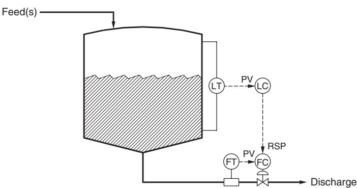
Introduce -- blocks, tags and finite resolution (Sec. 1.1-1.2)
- Input, output (valve) and control blocks; output named
<Tag>.<Attribute>, e.g.TC4011.SP. - Summer: $Y = k_0 + k_1X_1 + k_2X_2$. Moving average: $Y_k = \frac{1}{N}\sum_{j=0}^{N-1} X_{k-j}$.
- Temperatures are stored to 0.1 F resolution.
- Windup: "occurs when changes in the controller output have no effect on the process variable."
Code -- DCS blocks are one-line functions
- Summer and moving average, as Cecil writes them
np.round(x, 1)imitates the 0.1 F input resolution
def summer(X1, X2, k0=0.0, k1=1.0, k2=1.0):
    return k0 + k1 * X1 + k2 * X2

def moving_average(x, N):
    return np.convolve(x, np.ones(N) / N, mode="valid")

print(summer(120.0, 10.0, k2=-1.0))     # subtraction
print(np.round([107.43, 107.46], 1))    # 0.1 F resolution
110.0
[107.4 107.5]
Build on it -- resolution, and the cost of smoothing
- A slow 0.02 F/min ramp, measured at 0.1 F resolution
- Smoothing removes the staircase but adds lag
- For a ramp, an average over $T_A$ trails by $T_A/2$
t = np.arange(0, 60, 0.5)                  # min, sample 0.5 min
T_true = 107.0 + 0.02 * t                  # slow ramp
T_meas = np.round(T_true, 1)               # 0.1 F resolution
T_avg = moving_average(T_meas, 20)         # T_A = 10 min
lag = T_true[19:] - T_avg                  # true minus smoothed
print(f"steps in raw signal: {np.sum(np.diff(T_meas) != 0)}")
print(f"average lag of smoothed signal: {lag.mean():.3f} F")
steps in raw signal: 12
average lag of smoothed signal: 0.095 F
Build on it -- windup, as a logic statement
- Cecil's level-to-flow cascade: valve fully open gives 70 gpm
- Windup condition: output changes no longer move the PV
- Logic statements become Python booleans
def flow_from_valve(opening_pct, max_flow=70.0):
    return max_flow * min(opening_pct, 100.0) / 100.0

FC_SP = 85.0                              # set by the level ctrl
FC_MN = 100.0                             # flow ctrl output, %
FC_QH = FC_MN >= 100.0                    # at upper output limit
LC_TRKMR = FC_QH                          # Cecil: LC.TRKMR = FC.QH
print(flow_from_valve(FC_MN), "gpm; windup risk:", LC_TRKMR)
70.0 gpm; windup risk: True
Your Turn (8 min)
- By hand: a plant halves its scatter from $\sigma = 0.8$ to $0.4$ with $z = 2$. How far can the target move?
- Read the code: what does this print?
print(summer(50.0, 20.0, k0=5.0, k1=0.5, k2=2.0))
print(flow_from_valve(60.0))
Check -- cold-call
A plant asks: "why use override control instead of just tuning the PID harder?" Which of our two books answers that -- and why that one?
Wrap-up
Derived, then coded: the hot water tank under on/off, P and PI control; offset $e_{ss} = \Delta d/(1 + KK_c)$; apparent error and the gain limit; "narrow the variance, shift the target"; DCS blocks.
Tools: def, for loops (Euler steps), sp.solve, sp.limit,
np.clip, np.random, np.convolve
Next: Ch. 2-3 -- deriving the tank models we borrowed today, and solving them with Laplace transforms.